The abstract notion of duality is especially useful in stable homotopy theory because it interchanges homology and cohomology. Indeed, if \(X\) is a dualizable spectrum, then mapping out of \(X\) is equivalent to tensoring with its dual \(X^{\vee }\). Consequently, the cohomology of \(X\) can be computed as the homology of \(X^{\vee }\), and conversely the cohomology of \(X^{\vee }\) can be computed as the homology of \(X\). For spectra \(X\) and \(E\), we use the notation \[ E_k(X):=\pi _k(E\otimes X) \qquadtext {and} E^k(X):=\pi _{-k}\hom (X,E). \] For \(X=\S [A]\), this recovers the conventions for the \(E\)-(co)homology of an anima \(A\).
Lemma 11.3.1. Let \(X\) and \(E\) be spectra and assume that \(X\) is dualizable. Then there are natural isomorphisms \[ E_*(X^{\vee }) \cong E^{-*}(X) \qquadtext {and} E^*(X^{\vee }) \cong E_{-*}(X). \]
Proof. The first isomorphism follows from \[ E_*(X^{\vee }) \cong \pi _*(E \otimes X^{\vee }) \cong \pi _*(\hom (X,E)) \cong E^{-*}(X). \] The second follows by applying the first to \(X^{\vee }\), whose dual is \(X\). □
The dual of a dualizable spectrum is therefore also called its Spanier–Whitehead dual. The thick-subcategory property from Lemma 11.1.16 supplies the basic class of examples.
Proof. The category \(\Sp \) admits internal homs, the sphere spectrum is dualizable, and the dualizable spectra form a thick subcategory by Lemma 11.1.16. □
Proof. The collection of animae \(X\) for which \(\S [X]\) is dualizable is closed under finite colimits and contains \(* \in \An \); consequently it contains all finite animae. □
This gives an abstract existence result, but does not by itself identify the dual geometrically. For a closed smooth manifold, Atiyah duality provides such an identification in terms of the tangent bundle.
Let \(M\) be a closed smooth manifold of dimension \(n\), i.e. a compact smooth manifold without boundary. By Morse theory, \(M\) has the homotopy type of a finite CW-complex [Milnor (1963), Theorem 3.5 and Corollary 6.7]. It thus follows from Corollary 11.3.3 that its suspension spectrum \(\S [M]\) is dualizable. We will give an explicit description of its dual, due to Atiyah (1961): there is an isomorphism \[ D(\S [M]) \cong \th (-T_M) \] between the dual of \(\S [M]\) and the Thom spectrum of the negative stable tangent bundle \(-T_M\). Here \(-T_M\) denotes the inverse of the virtual vector bundle \([T_M]\) of Example 10.2.20, which has rank \(-n\), and \(\th (-T_M)\) is its Thom spectrum in the sense of Construction 10.2.16. No new construction is required: the group completion entering the stable J-homomorphism already assigns a Thom spectrum to every virtual vector bundle, of any rank.
To get a better understanding of the Thom spectrum \(\th (-T_M)\), we will now show that we can write it as \(\Sigma ^{\infty - N}(\Th (\nu _{\phi }))\) for a suitable honest vector bundle \(\nu _{\phi }\) over \(M\). The main ingredient is the following simple observation:
Lemma 11.3.4. Let \(M\) be a compact smooth \(n\)-manifold. Then there exists a natural number \(N\) and a smooth embedding \(\phi \colon M \hookrightarrow \R ^N\).
Proof. By compactness, we may choose finitely many coordinate charts \(\phi _i\colon U_i \to \R ^n\), smaller open subsets \(V_i\) which still cover \(M\) and satisfy \(\overline {V_i}\subseteq U_i\), and smooth functions \(\rho _i\colon M \to [0,1]\) supported in \(U_i\) and strictly positive on \(V_i\). Extend \(\rho _i\phi _i\) by zero outside \(U_i\) and consider \[ \phi := (\rho _i\phi _i,\rho _i)_{i=1}^k\colon M \longrightarrow (\R ^n \times \R )^k. \] If \(x \neq y\), choose \(i\) with \(x \in V_i\). Equality of the \(i\)th pair of coordinates would force \(\rho _i(y)=\rho _i(x)>0\), hence \(y\in U_i\), and then \(\phi _i(y)=\phi _i(x)\), a contradiction. Thus \(\phi \) is injective. The same coordinate pair shows that \(d\phi \) is injective at \(x\): if it killed a tangent vector, then both \(d\rho _i\) and \(d(\rho _i\phi _i)=\rho _i d\phi _i+\phi _i d\rho _i\) would vanish, and hence so would \(d\phi _i\). Thus \(\phi \) is an injective immersion. Since \(M\) is compact, it is a smooth embedding. □
Remark 11.3.5. If \(n>0\), the Whitney embedding theorem shows that \(N\) can be chosen to be \(2n\) in the previous lemma.
For the remainder of this section, we will fix once and for all a smooth embedding \(\phi \colon M \hookrightarrow \R ^N\). We will denote by \(\nu := \nu _{\phi } \to M\) the normal bundle of this embedding, i.e., the cokernel of the map \(T_M \to \phi ^*(T_{\R ^N}) \cong \ul {\R ^N}\) of vector bundles over \(M\): \[ T_M \to \ul {\R ^N} \to \nu . \] By choosing a metric on the vector bundle \(\ul {\R ^N}\) one obtains an orthogonal decomposition \[ \ul {\R ^N} \cong T_M \oplus \nu . \] Passing to classes of virtual vector bundles and using Example 10.2.20, this gives \([T_M] + [\nu ] \cong [\ul {\R ^N}]\), so that \(-T_M\) is the virtual vector bundle \([\nu ] - [\ul {\R ^N}]\) of rank \(-n\). Hence Lemma 10.2.21 identifies \begin {equation} \label {eq:Thom_Spectrum_Negative_Tangent_Bundle} \th (-T_M) \cong \th (\nu )[-N] \cong \Sigma ^{\infty - N}(\Th (\nu )). \end {equation}
We will now construct the duality data exhibiting \(\th (-T_M)\) as dual to \(\S [M]\). In the order fixed by Definition 11.1.1, these are maps \[ \ev \colon \th (-T_M)\otimes \S [M]\to \S \qquadtext {and} \coev \colon \S \to \S [M]\otimes \th (-T_M) \] satisfying the triangle identities. Using Equation 11.1, it is enough to construct maps of pointed spaces \[ \Th (\nu )\wedge M_+\to S^N \qquadtext {and} S^N\to M_+\wedge \Th (\nu ). \] The constructions below naturally produce these maps with the two smash factors reversed. We use the symmetry of the smash product to put them in the displayed order, but suppress these symmetry maps in the point-set formulas. We will use Thom-space functoriality and the Pontryagin–Thom collapse map.
Construction 11.3.6. Let \(f\colon X \to Y\) be a continuous map of topological spaces. Let \(p\colon E \to Y\) be a vector bundle over \(Y\), and let \(f^*(E) \to X\) be its pullback bundle. By applying functoriality of the Thom space construction (Construction 10.1.7) to the commutative diagram
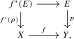
we obtain a continuous map \[ f_*\colon \Th (f^*E) \to \Th (E). \]
Example 11.3.7. Consider the terminal map \(p\colon M \to \pt \), and consider the trivial vector bundle \(E = \R ^N \to \pt \). Then the pullback bundle \(p^*(\R ^N)\) is the trivial vector bundle \(\ul {\R ^N}\) over \(M\), and we obtain a map \[ p_*\colon \Sigma ^N(M_+) \overset {\text{Example 10.1.5}}{\cong } \Th (\ul {\R ^N}) \xrightarrow {p_*} \Th (\R ^N) \overset {\text{Example 10.1.5}}{\cong } S^N. \]
Example 11.3.8. Consider the diagonal map \(\Delta \colon M \to M \times M\), and let \(E = \nu \times \ul {0}\) be the product bundle over \(M \times M\), where \(\nu \) is the normal bundle of our fixed embedding \(\phi \colon M \hookrightarrow \R ^N\) and \(\ul {0}\) is the zero bundle. Observe that the pullback bundle \(\Delta ^*(E) = \Delta ^*(\nu \times \ul {0})\) is isomorphic to the direct sum \(\nu \oplus \ul {0}\) of these two bundles, and hence is isomorphic to \(\nu \) itself. The above construction thus produces a map \[ \Delta _*\colon \Th (\nu ) \to \Th (\nu \times \ul {0}) \overset {\text{Example 10.1.6}}{\cong } \Th (\nu ) \wedge \Th (\ul {0}) \cong \Th (\nu ) \wedge M_+. \]
Recall the Pontryagin–Thom collapse map \(\PT (i)\colon N'_+ \to \Th (\nu (i))\) of Construction 10.1.8. We will also need the following twisted version.
Construction 11.3.9 (Twisted Pontryagin-Thom collapse map). The Pontryagin-Thom collapse map also has a ‘twisted’ version, where in addition to a smooth embedding \(i\colon N \hookrightarrow N'\) of compact manifolds without boundary we are given a vector bundle \(E\) over \(N'\). It takes the form \[ \PT (i,E)\colon \Th (E) \to \Th (\nu (i) \oplus i^*E). \] To define it, choose a metric on \(E\) and consider the composite embedding \(N \xhookrightarrow {i} N' \xhookrightarrow {s_0} E\), where the second map is the zero-section. Its normal bundle is the direct sum \(\nu (i) \oplus i^*E\), so the ordinary Pontryagin–Thom construction gives a collapse map \[ E_+ \longrightarrow \Th (\nu (i) \oplus i^*E). \] We may choose its tubular neighborhood inside the open unit disk bundle of \(E\). The collapse map then sends the complement of that disk bundle, and in particular the unit sphere bundle, to the basepoint. It therefore factors through the quotient \(E_+ \to E^+\cong \Th (E)\) of Remark 10.1.4, giving the desired twisted collapse map. Its based homotopy class is independent of the metric and tubular-neighborhood choices.
Example 11.3.10. Consider our fixed embedding \(\phi \colon M \hookrightarrow \R ^N\). Since \(M\) is compact, its image is closed in \(S^N\) and misses the point at infinity. Thus \(M\hookrightarrow S^N\) is a pointed smooth embedding, and the Pontryagin-Thom construction provides a map \[ \PT (\phi )\colon S^N \to \Th (\nu ). \]
Example 11.3.11. Consider the diagonal embedding \(\Delta \colon M \hookrightarrow M \times M\). Its normal bundle is isomorphic to the tangent bundle \(T_M\) of \(M\). As a twist, we use the external direct sum \(E = \ul {0} \times \nu \) over \(M \times M\), where \(\nu = \nu (\phi )\) as before. The pullback of \(E\) along \(\Delta \) is isomorphic to \(\nu \), as in Example 11.3.8, and we see that there is a trivialization \(\nu (\Delta ) \oplus \Delta ^*(E) \cong T_M \oplus \nu \cong \ul {\R ^N}\). The twisted Pontryagin-Thom map in this case takes the form \[ \PT (\Delta ,\ul {0} \times \nu )\colon M_+ \wedge \Th (\nu ) \cong \Th (\ul {0}) \wedge \Th (\nu ) \cong \Th (\ul {0} \oplus \nu ) \to \Th (\ul {\R ^N}) \cong \Sigma ^N(M_+). \]
Combining the four examples, we obtain our evaluation and coevaluation maps: \[ \ev \colon M_+ \wedge \Th (\nu ) \xrightarrow {\PT (\Delta , \ul {0} \times \nu )} \Sigma ^N(M_+) \xrightarrow {p_*} \Sigma ^N(S^0) = S^N. \] \[ \coev \colon S^N \xrightarrow {\PT (\phi )} \Th (\nu ) \xrightarrow {\Delta _*} \Th (\nu ) \wedge M_+. \]
To finish the proof of Atiyah duality, it remains to show that these maps satisfy the space-level analogues of the triangle identities. We will use the following standard compatibilities of the Pontryagin–Thom construction. We formulate them only for compact manifolds without boundary, which is the case needed below.
Proposition 11.3.12 (Pontryagin–Thom calculus). Pontryagin–Thom collapse maps have the following properties, up to based homotopy.
- (1)
-
Isotopy invariance. Isotopic embeddings induce homotopic collapse maps. The same holds for twisted collapse maps, provided the twisting bundle is fixed throughout the isotopy.
- (2)
-
Compatibility with composition. Let \(N \xhookrightarrow {i} P \xhookrightarrow {j} Q\) be smooth embeddings of compact manifolds, and let \(E\) be a vector bundle over \(Q\). After choosing a splitting of the normal-bundle sequence \[ 0 \to \nu (i) \to \nu (ji) \to i^*\nu (j) \to 0, \] the composite \[ \Th (E) \xrightarrow {\PT (j,E)} \Th (\nu (j) \oplus j^*E) \xrightarrow {\PT (i,\nu (j)\oplus j^*E)} \Th (\nu (i) \oplus i^*\nu (j) \oplus (ji)^*E) \] agrees up to homotopy with \(\PT (ji,E)\) under the resulting identification of target Thom spaces.
- (3)
-
Transverse base change. Let \(f\colon M_1 \to M_2\) be a smooth map between compact smooth manifolds without boundary and let \(i_2\colon N_2 \hookrightarrow M_2\) be a closed smooth submanifold. Assume that \(f\) is transverse to \(N_2\), and set \(N_1 := f^{-1}(N_2)\), with inclusion \(i_1\colon N_1 \hookrightarrow M_1\) and induced map \(\bar f\colon N_1 \to N_2\). Then \(N_1\) is a smooth submanifold and there is a natural isomorphism \(\nu (i_1) \cong \bar f^*\nu (i_2)\). Under this identification, the square
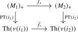
commutes up to based homotopy. More generally, for a vector bundle \(E\) over \(M_2\), the square
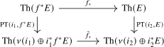
commutes up to based homotopy.
Proof sketch. Choose Riemannian metrics and tubular neighborhoods. An isotopy of embeddings has a tubular neighborhood over the parameter interval, which gives the homotopy in (1). For (2), choose nested tubular neighborhoods for \(N \subseteq P \subseteq Q\); collapsing successively then agrees with collapsing the resulting tubular neighborhood of \(N\) in \(Q\). For (3), transversality identifies the normal bundle of \(N_1\) with \(\bar f^*\nu (i_2)\). Compactness allows the tubular neighborhoods to be chosen compatibly over the whole square. Comparing the corresponding collapse quotients gives the displayed homotopies. The same choices made in the total space of \(E\) prove the twisted statements. □
We are finally ready to prove Atiyah duality. Consider the composite \begin {align*} \th (-T_M)\otimes \S [M] &\cong \Sigma ^{\infty -N}\Th (\nu )\otimes \S [M] \cong \Sigma ^{\infty -N}(\Th (\nu )\wedge M_+) \\ &\cong \Sigma ^{\infty -N}(M_+\wedge \Th (\nu )) \\ &\xrightarrow {\Sigma ^{\infty - N}\PT (\Delta , \ul {0} \times \nu )} \Sigma ^{\infty - N}\Sigma ^N(M_+) \\ &\xrightarrow {p_*} \Sigma ^{\infty - N}\Sigma ^N(S^0) \cong \S . \end {align*}
Its homotopy class is independent of the metrics and tubular neighborhoods used in its construction.
Theorem 11.3.13 (Atiyah duality). The displayed map exhibits \(\th (-T_M)\) as a dual of \(\S [M]\), and hence determines an isomorphism: \[ D(\S [M])\cong \th (-T_M). \]
Proof. We verify the triangle identities before applying suspension spectra. Each triangle composite is built from twisted collapse maps and a Thom-space pushforward. Transverse base change rewrites it as the composite of a collapse map for a graph embedding and the pushforward along an identity map. Compatibility with composition and isotopy invariance then identify both factors with identity maps.
Observe that the map we wrote is obtained by applying \(\Sigma ^{\infty -N}(-)\colon \Top _* \to \An _* \to \Sp \) to the following composite: \[ \ev \colon M_+ \wedge \Th (\nu ) \xrightarrow {\PT (\Delta , \ul {0} \times \nu )} \Sigma ^N(M_+) \xrightarrow {p_*} \Sigma ^N(S^0) = S^N. \] For the candidate coevaluation map, we similarly apply \(\Sigma ^{\infty - N}(-)\) to the following composite: \[ \coev \colon S^N \xrightarrow {\PT (\phi )} \Th (\nu ) \xrightarrow {\Delta _*} \Th (\nu ) \wedge M_+. \] To see that the triangle identities are satisfied, it is enough to prove corresponding homotopies at the level of topological spaces. More precisely, the triangle identity on \(\th (-T_M)\) is obtained by applying \(\Sigma ^{\infty -2N}\) to the composite \[ S^N \wedge \Th (\nu ) \xrightarrow {\coev \wedge \id } \Th (\nu ) \wedge M_+ \wedge \Th (\nu ) \xrightarrow {\id \wedge \ev } \Th (\nu ) \wedge S^N \] while the triangle identity on \(\S [M]\) is obtained by applying \(\Sigma ^{\infty -N}\) to \[ M_+ \wedge S^N \xrightarrow {\id \wedge \coev } M_+ \wedge \Th (\nu ) \wedge M_+ \xrightarrow {\ev \wedge \id } S^N \wedge M_+ \] Thus it suffices to show that these two composites are homotopic to the respective identities, up to the displayed symmetries of the smash product. We will start with the former. Consider the following pullback square:
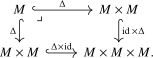
Let us check the transversality hypothesis in this instance. At a point \((x,y)\) of the inverse image of \(\im (\id \times \Delta )\), the image of \(d(\Delta \times \id )\) consists of triples \((v,v,w)\), while the tangent space to \(\im (\id \times \Delta )\) consists of triples \((a,b,b)\). Every triple \((r,s,t)\) decomposes as \[ (r,s,t)=(s,s,t)+(r-s,0,0), \] with the first summand of the former type and the second of the latter type. Thus \(\Delta \times \id \) is transversal to \(\im (\id \times \Delta )\). Applying Proposition 11.3.12 to this square (i.e. we take \(M_2 := M \times M \times M\), \(N_2 := M \times M\), \(i_2 = \id \times \Delta \), \(M_1 := M \times M\), \(N_1 := M\), \(f = \Delta \times \id \) and \(E = \nu \times \ul {0} \times \nu \)) gives the following homotopy-commutative diagram:
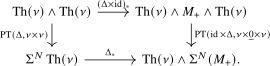
All collapse maps below whose source contains \(S^N_+\) factor through the reduced quotient, since the relevant embeddings lie in \(\R ^N\times M\). We use these reduced maps without further notation. Unwinding the definitions of \(\coev \wedge \id \) and \(\id \wedge \ev \), we then get the following homotopy-commutative diagram. Its top row is the triangle composite, its southeast-pointing arrows are Pontryagin–Thom collapse maps, and its northeast-pointing arrows are Thom-space pushforwards:
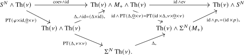
The upper two triangles commute by the definitions of \(\coev \) and \(\ev \), while the central diamond is the transverse base-change square displayed above. By compatibility with composition in Proposition 11.3.12, the left diagonal composite is induced on the reduced quotient by the twisted Pontryagin–Thom collapse map for the composite \[ j\colon M \xhookrightarrow {\Delta } M \times M \xhookrightarrow {\phi \times \id } S^N \times M, \] where we twist by the bundle \(\ul {0} \times \nu \) on \(S^N \times M\). The corresponding unreduced twisted collapse map is \[ \PT (j,\ul {0} \times \nu )\colon S^N_+ \wedge \Th (\nu ) \to \Sigma ^N\Th (\nu ), \] Since the image of \(j\) is contained in \(\R ^N \times M \subseteq S^N \times M\), this map collapses the entire fiber over the point at infinity and therefore factors through the quotient \(S^N_+ \wedge \Th (\nu ) \twoheadrightarrow S^N \wedge \Th (\nu )\). The embedding \(j=(\phi ,\id )\) is isotopic, via the straight-line isotopy in \(\R ^N \subseteq S^N\), to the embedding \((0,\id )\colon M \hookrightarrow \R ^N \times M \subseteq S^N \times M\). By isotopy invariance, the induced map on the reduced quotient is therefore homotopic to the one obtained from \((0,\id )\). Using \(\R ^N \times M\) as a tubular neighborhood for this inclusion, we see that the latter is the identity on \(S^N \wedge \Th (\nu )\).
The right diagonal is the pushforward functoriality of Thom spaces applied to the composite \[ M \xhookrightarrow {\Delta } M \times M \xrightarrow {\id \times p} M \times \pt = M. \] But this composite is simply the identity on \(M\), hence it induces the identity on \(S^N \wedge \Th (\nu )\). We conclude that the composite \((\id \wedge \ev ) \circ (\coev \wedge \id )\) is homotopic to the identity on \(S^N \wedge \Th (\nu )\), proving the first triangle identity.
The second triangle identity follows by the same argument, applied to the transposed pullback square. More precisely, we now take \(i_2 = \Delta \times \id \), \(f = \id \times \Delta \) and use the twist \(E = \ul {0} \times \nu \times \ul {0}\) over \(M \times M \times M\). Transverse base change and compatibility with composition identify the composite \((\ev \wedge \id ) \circ (\id \wedge \coev )\) with the composite of the Pontryagin–Thom collapse map for the graph embedding \[ (\id ,\phi )\colon M \hookrightarrow M \times S^N \] and the Thom-space pushforward induced by \((p \times \id ) \circ \Delta = \id _M\). The graph embedding is isotopic to \((\id ,0)\colon M \hookrightarrow M \times \R ^N\), whose collapse map is the identity on \(M_+ \wedge S^N\) under the standard Thom identifications. Hence the second triangle composite is also homotopic to the identity. □
Generated from the authoritative LaTeX source.