Recall that a monoid is a set \(M\) equipped with a unit element \(1 \in M\) and a product \(x \cdot y \in M\) for all \(x, y \in M\), satisfying associativity and unitality. Given such a monoid, we obtain for every \(n \geq 0\) an \(n\)-fold multiplication map \(M^n \to M\) sending \((x_1, \ldots , x_n)\) to \(x_1 \cdots x_n\). In the \(\infty \)-categorical setting, we make all these \(n\)-fold multiplication maps part of the data, together with all the coherences between them. These coherences are encoded by the simplex category \(\simp \).
Definition 5.1.1 (Monoid). Let \(C\) be an \(\infty \)-category that admits finite products. We define a monoid object in \(C\) (or \(E_1\)-monoid) to be a simplicial object \[ M\colon \simp \catop \to C, \qquad [n] \mapsto M_n := M([n]), \] satisfying the Segal condition: for every \([n] \in \simp \) the Segal map \[ (e_i^*)_{i=1}^n \colon M_n \to \prod _{i=1}^n M_1 \] induced by the \(n\) inclusion maps \(e_i \colon [1] \cong \{i-1 \leq i \} \hookrightarrow [n]\) is an isomorphism. In particular, the condition for \(n = 0\) requires \(M_0\) to be a terminal object of \(C\). We write \[ \Mon (C) \subseteq \Fun (\simp \catop ,C) \] for the full subcategory spanned by the monoids in \(C\). We refer to \(M_1\) as the underlying object of \(M\).
Convention 5.1.2. Given a monoid \(M\), we will often denote its underlying object in \(C\) again by \(M\). We will also often identify \(M_n\) with the \(n\)-fold product \(M^n := \prod _{i=1}^n M\) via the Segal map.
The unique map \(s^0\colon [1] \to [0]\) and the inclusion \(d^1\colon [1] \cong \{0 \leq 2\} \hookrightarrow [2]\) in \(\simp \) induce maps \(M_0 \to M_1\) and \(M_2 \to M_1\), which under our convention take the form \[ e\colon * \to M \quad \qquadtext { and } \quad m\colon M \times M \to M. \] We refer to \(e\) as the unit or neutral element of \(M\), and refer to \(m\) as the multiplication of \(M\). The unitality and associativity of multiplication are encoded by the following commutative diagrams in \(\simp \), where we denote an order-preserving map \([m] \to [n]\) by listing the images \((a_0, \ldots , a_m)\) of the elements \(0, \ldots , m\):
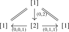
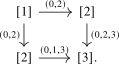
Similarly, all the expected ‘higher coherences’ relating the various ways of multiplying four, five, or more elements in \(M\) follow from suitable higher dimensional diagrams in \(\simp \). More explicitly, for a map \(\phi \colon [m] \to [n]\) in \(\simp \) we should think of the resulting map \(\phi ^*\colon M^n \to M^m\) as follows: \[ \phi ^*(x_1, \dots , x_n) := (y_1, \dots , y_m), \qquad \qquad y_i := \prod _{\phi (i-1) < j \leq \phi (i)} x_j. \] This formula becomes transparent once we think of the elements \(x_1, \dots , x_n\) as labels on the \(n\) inequalities of \([n]\), and likewise of \(y_1, \dots , y_m\) as labels on the \(m\) inequalities of \([m]\). Drawing the map \(\phi \) then cuts the strip between \([m]\) and \([n]\) into \(m\) blocks, one for each inequality of \([m]\), and the label of an inequality of \([m]\) is the product of the labels it sees in its block. For \(\phi \colon [4] \to [5]\) with \(\phi (0) = 0\), \(\phi (1) = \phi (2) = 2\), \(\phi (3) = 4\) and \(\phi (4) = 5\) this looks as follows:
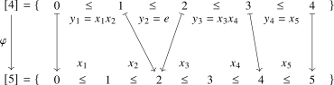
The \(i\)-th block is bounded by the arrows starting at \(i-1\) and at \(i\), so the inequalities of \([5]\) it contains are exactly those indexed by \(\phi (i-1) < j \leq \phi (i)\); multiplying their labels gives \(y_i\). Note that the strip is read against the direction of \(\phi \): the labels travel from \([5]\) up to \([4]\), which is precisely the contravariance of \(M\). Since \(\phi (1) = \phi (2)\), the two arrows bounding the second block meet at \(2\), so this block contains no inequality of \([5]\) at all; its label is therefore the empty product, that is, the unit \(e\). In this example we thus obtain \[ \phi ^*(x_1, \dots , x_5) = (x_1x_2, \; e, \; x_3x_4, \; x_5). \]
Exercise 5.1.3. Let \(F\colon C \to D\) be a functor preserving finite products. Show that \(F\) induces a functor \(\Mon (C) \to \Mon (D)\).
Example 5.1.4. By Chapterexercise 5.1, a topological monoid is a monoid object in \(\Top \). Combining the preceding exercise with the fact that \(\Pi _{\infty }\colon \Top \to \An \) preserves finite products (see Corollary 2.3.20), we see that every topological monoid \(M\) defines a monoid object \(\Pi _{\infty }(M)\) in \(\An \).
Definition 5.1.5. We say that a monoid \(M \in \Mon (C)\) is grouplike, or a group in \(C\), if the so-called shear map \[ (\pr _1,m)\colon M \times M \to M \times M, \qquad (x,y) \mapsto (x,xy) \] is an isomorphism in \(C\). We denote by \(\Grp (C) \subseteq \Mon (C)\) the full subcategory spanned by the groups in \(C\).
Exercise 5.1.6. Show that a monoid \(M \in \Mon (\Set )\) is a group in the sense of Definition 5.1.5 if and only if every element \(x\) admits an inverse \(x^{-1}\).
Exercise 5.1.7. For a group object \(G \in \Grp (C)\), construct an inverse map \((-)^{-1}\colon G \to G\) in \(C\).
5.1.1 Group structures on loop spaces
We will now introduce a general class of examples of group objects in \(\infty \)-categories: the loop objects \(\Omega X\) on pointed objects \(X\). If \(C\) is an \(\infty \)-category with finite limits, then we may apply Chapterexercise 4.3 in the pointed \(\infty \)-category \(C_*\) to obtain a group structure on \(\Omega X\) in \(\Ho (C_*)\), and hence in \(\Ho (C)\). We will now explain how to lift this structure to a group structure in \(C\).
Let us first explain informally where the multiplication on \(\Omega X\) comes from. The loop object is defined as the pullback \(\Omega X = * \times _X *\); for \(C = \An \), its points are the loops in \(X\) at the basepoint \(x\). Multiplication should be given by composing loops, and it is the universal property of pullbacks that produces this map for us: consider the iterated pullback \(* \times _X * \times _X *\), which comes with three natural projections to \(* \times _X *\). Projecting away the third or the first factor yields two maps which exhibit the iterated pullback as the product \(\Omega X \times \Omega X\), as verified in Lemma 5.1.13. Projecting away the middle factor instead yields a map \[ m\colon \Omega X \times \Omega X \to \Omega X, \] and this is composition of loops. Similarly, the universal property of the pullback \(\Omega X = * \times _X *\) turns the constant homotopy at the basepoint into a unit map \(e\colon * \to \Omega X\), the constant loop.
The higher coherences arise from the same principle. The \((n+1)\)-fold iterated pullback \(* \times _X \dots \times _X *\) is the object of \(n\)-tuples of composable loops, and projecting away some of the inner factors realizes all the ways of composing consecutive loops in such a tuple. For example, associativity compares the two ways of composing three loops, and both are obtained from projections \(* \times _X * \times _X * \times _X * \to * \times _X *\) which forget the two inner factors one at a time; the universal property identifies both composites with the projection onto the two outer factors. Rather than listing such coherences one at a time, we should remember the entire family of iterated pullbacks together with all projections between them, as well as the maps which repeat a factor and correspond to inserting a constant loop. This is precisely the structure of a simplicial object satisfying the Segal condition: face maps compose loops, and degeneracy maps insert constant loops.
It remains to construct this simplicial object, with all its coherences, functorially from the basepoint map \(x\colon * \to X\). This will be achieved by a right Kan extension, indexed by the following enlargement of the simplex category.
Definition 5.1.8. We define the augmented simplex category as \(\simp _+ := \simp ^{\triangleleft }\), the cone of the simplex category. We denote the cone point by \([-1]\). A functor \(\simp _+\catop \to C\) is called an augmented simplicial object. It corresponds to a simplicial object \(X_{\bullet }\colon \simp \catop \to C\) equipped with a cocone \(X_{\bullet } \Rightarrow \const _{X_{-1}}\).
Note that we may identify \(\simp _+\) with the full subcategory of the category \(\Poset \) of posets spanned by the linearly ordered sets \([n] = \{0 \leq \dots \leq n\}\), where we set \([-1] = \emptyset \). There are fully faithful inclusions \[ i\colon \simp \hookrightarrow \simp _+ \quad \qquadtext { and } \quad j\colon [1] \hookrightarrow \simp _+, \quad j(0) = [-1], \quad j(1) = [0]. \]
Definition 5.1.9. Let \(C\) be an \(\infty \)-category with pullbacks. We define the Čech nerve functor \(\check {C}\colon \Ar (C) \to \Fun (\simp \catop ,C)\) as the composite \[ \check {C}_{\bullet }\colon \Ar (C) \simeq \Fun ([1]\catop ,C) \xrightarrow {j_*} \Fun (\simp _+\catop ,C) \xrightarrow {i^*} \Fun (\simp \catop ,C), \] where \(j_*\) is the right Kan extension functor along the inclusion \(j\catop \colon [1]\catop \hookrightarrow \simp _+\catop \), and where \(i^*\) is restriction along the inclusion \(i\catop \). Given a morphism \(f\colon X \to Y\) in \(C\), we refer to the simplicial object \(\check {C}_{\bullet }(f)\) as the Čech nerve of \(f\).
Here the equivalence \(\Ar (C) \simeq \Fun ([1]\catop ,C)\) uses the order-reversing isomorphism \([1] \cong [1]\catop \): a morphism \(f\colon X \to Y\) corresponds to the functor with value \(X\) at \(1\) and \(Y\) at \(0\). In the pointwise calculation below, we use the same order reversal to write it in the usual form \(f\colon [1] \to C\), with \(f(0)=X\) and \(f(1)=Y\).
For a discussion of the theory of Kan extensions, we refer the reader to Section 21.4.
Discussion 5.1.10. The existence of the right adjoint \(j_*\) to \(j^*\) follows from the pointwise formula for Kan extensions from Theorem 21.4.3. Given a morphism in \(C\) of the form \(f\colon [1] \to C\), the pointwise formula says that the value of \(j_*(f)\colon \simp \catop _+ \to C\) at \([n] \in \simp _+\) is given by the limit \(\lim _{I_n} f_n\), where \(I_n\) is the full subcategory of the slice \(((\simp _+)_{/[n]})\catop \) spanned by all objects of the form \([-1] \to [n]\) and \([0] \to [n]\), and where \(f_n\) is the composite \(I_n \to [1] \xrightarrow {\smash {f}} C\). Since there is a unique map \(\infty \colon [-1] \to [n]\) and there is one map \(i\colon [0] \to [n]\) for every \(0 \leq i \leq n\), the category \(I_n\) may be identified with the following poset:
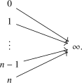
The forgetful functor \(I_n \to [1]\) sends \(\infty \) to \(1\) and sends each \(0 \leq i \leq n\) to \(0\). In particular, the functor \(f_n\colon I_n \to C\) takes the form
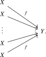
Since \(C\) admits pullbacks, the limit of this diagram exists in \(C\) and is given by the \((n+1)\)-fold fiber product of \(X\) with itself over \(Y\). All in all, we see that the Čech nerve of a morphism \(f\colon X \to Y\) in \(C\) is well-defined and is given in degree \(n\) by \[ \check {C}_n(f) \quad \simeq \quad X^{\times ^{n+1}_Y} \quad = \quad X \times _{Y} X \times _{Y} \dots \times _Y X. \]
Definition 5.1.11 (Loop group). Let \(C\) be an \(\infty \)-category with finite limits. We define the loop group \(\bOmega (X,x) \in \Fun (\simp \catop ,C)\) of a pointed object \((X,x)\) in \(C\) as the Čech nerve of the morphism \(x\colon * \to X\). This results in a functor \(\bOmega \colon C_* \to \Fun (\simp \catop ,C)\).
Remark 5.1.12. Since the loop object \(\Omega (X,x)\) is defined as the pullback \(* \times _X *\) in \(C\), there is a natural isomorphism \[ \bOmega (X,x)_1 \cong \Omega (X,x), \] justifying the notation.
Lemma 5.1.13. For every pointed object \(X\), the loop group \(\bOmega X\) is a group object in \(C\).
Proof. To show that \(\bOmega X\) is a monoid, we will show by induction that for every \(n\) the map \[ (e_i^*)_{i=1}^n\colon (\bOmega X)_n \to \prod _{i=1}^n \Omega X \] is an isomorphism in \(C\). For \(n = 0\), observe that \(I_0\) is isomorphic to the walking morphism \([1]\), consisting of objects \(0\) and \(\infty \), and the functor \(f_0\colon I_0 \to C\) is the diagram \(* \to X\). Since \([1]\) has \(0\) as an initial object, this limit is simply \(*\); see Lemma 21.2.4. The case \(n=1\) is the identification from the preceding remark. For \(n \geq 1\), note that we may write \(I_{n+1}\) as a pushout of \(I_n\) and \(I_1\) along \(I_0\):

By applying Theorem 21.2.11(2) with \(J = \,\,\pushout \), we thus obtain a pullback square of the form
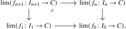
where we take \(f\) to be the basepoint map \(x\colon * \to X\). By induction, this pullback square is isomorphic to the commutative square
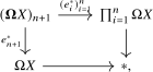
and so this being a pullback square means that the map \((\bOmega X)_{n+1} \xrightarrow {(e_i^*)_{i=1}^{n+1}} \prod _{i=1}^{n+1} \Omega X\) is an isomorphism, finishing the induction step. This shows that \(\bOmega X \) is a monoid in \(C\).
To see that \(\bOmega X\) is grouplike, write \(p_{ij}\colon * \times _X * \times _X * \to * \times _X *\) for the projection retaining the \(i\)-th and \(j\)-th factors. Under the Segal isomorphism \[ (p_{01},p_{12})\colon * \times _X * \times _X * \iso \Omega X \times \Omega X, \] the shear map is identified with \((p_{01},p_{02})\). But associativity of pullbacks gives another isomorphism \[ (p_{01},p_{02})\colon * \times _X * \times _X * \iso (* \times _X *) \times _* (* \times _X *) \cong \Omega X \times \Omega X. \] Thus the shear map is an isomorphism. □
5.1.2 Classifying animae
The loop group functor admits a left adjoint:
Construction 5.1.14 (Classifying anima of a monoid). Let \(C\) be an \(\infty \)-category admitting finite products and geometric realizations. Given a monoid \(M\), we define its classifying anima \(\bB M\) as \[ \bB M \quad := \quad \abs {M} \quad = \quad \colim _{[n] \in \simp \catop } M_n \qin C. \] We may turn this into a pointed object in \(C\) via the map \(* = M_0 \to \colim _{[n] \in \simp \catop } M_n\). This construction is functorial in \(M\), resulting in a functor \(\bB \colon \Mon (C) \to C_*\).
Proposition 5.1.15. Assume that \(C\) admits both finite limits and geometric realizations. Then the functors \(\bB \) and \(\bOmega \) define adjunctions \[ \bB \colon \Mon (C) \rightleftarrows C_* \noloc \bOmega \qquadtext { and } \bB \colon \Grp (C) \rightleftarrows C_* \noloc \bOmega . \]
Proof. Consider the following two adjunctions:

The bottom composite \(i^*j_*\) is precisely the Čech nerve functor \(\check {C}_{\bullet }\). The functor \(i_!\) is given by left Kan extension along \(i\). From the pointwise formula for left Kan extensions, we see that the top composite \(j^*i_!\) sends a simplicial object \(X\) in \(C\) to the map \(X_0 \to \abs {X} = \colim _n X_n\).
Now, note that the top composite \(j^*i_!\) sends the full subcategory \(\Mon (C) \subseteq \Fun (\simp \catop ,C)\) into the full subcategory \(C_* \subseteq \Ar (C)\), and that the resulting functor \(\Mon (C) \to C_*\) is precisely \(\bB \). Similarly, the bottom composite \(i^*j_*\) restricts to \(\bOmega \colon C_* \to \Mon (C)\). It follows that the adjunction \(j^*i_! \dashv i^*j_*\) restricts to an adjunction \(\bB \dashv \bOmega \) between \(\Mon (C)\) and \(C_*\). Since \(\bOmega \) takes values in \(\Grp (C) \subseteq \Mon (C)\), this adjunction further restricts to an adjunction between \(\Grp (C)\) and \(C_*\). □
For later use, we record the following observation:
Lemma 5.1.16. The classifying anima functor \(\bB \colon \Mon (\An ) \to \An \) preserves finite products.
Proof. This functor factors as \[ \Mon (\An ) \hookrightarrow \sAn \xrightarrow {\abs {-}} \An . \] The geometric realization functor \(\abs {-}\) preserves finite products by Lemma 21.6.12, and the inclusion preserves finite products since monoids are closed under products in \(\sAn \). □
Generated from the authoritative LaTeX source.